In the high-stakes world of Enrollment Management, we often describe our work as a blend of art and science. The “art” is undeniable; it is found in the warmth of a campus tour, the design of a viewbook, and the personalized counseling provided to anxious families. However, the “science” component is often relegated to simple spreadsheets and historical averages. This approach leaves a massive strategic advantage on the table. The true science of our profession is Probability Theory.

Every time a Vice President predicts a class size, a Director calculates a yield rate, or a marketing manager segments a search buy, they are engaging in a probabilistic experiment. To move beyond “gut feeling” and build sophisticated predictive models—such as the Markov Chains we will discuss later in this book—we must first master the fundamental mechanics of chance. This chapter translates the abstract definitions of a statistics textbook into the concrete strategies of the admissions funnel.

The Admissions Cycle as an Experiment

In the lexicon of statistics, an experiment is defined as any process of trial and observation where the outcome is uncertain before it is performed.

For an enrollment manager, the “experiment” is nothing less than the entire Admissions Cycle. When you launch your application on August 1st, you are initiating a massive, complex experiment. You have hypotheses and historical data, but the final result—the exact number of students sitting in seats on Census Day—is a random variable that will not be fully realized until the cycle closes.

To make sense of this uncertainty, we must define our Sample Space. Mathematically denoted by the symbol Ω, the sample space is the collection of all possible elementary outcomes. In your world, the Sample Space represents your Total Prospect Pool. If you purchase 100,000 names from the College Board and add them to your CRM, your sample space consists of those 100,000 specific individuals. Each student is a “sample point,” a distinct unit of data that will eventually take a path through your funnel.

Within this massive pool, we track Events.

An event is simply a subset of the sample space, the occurrence of a prescribed outcome. “Becoming an Inquiry” is an event. “Submitting an application” is an event. “Melting over the summer” is an event. The power of probability comes from analyzing how these events interact. We use set theory to describe these interactions.

Consider your segmentation strategy. You might be looking for students who fit a specific profile. 

The Intersection of events (A∩B) describes outcomes that share commonalities. If Event A represents “Students with a 3.8 GPA” and Event B represents “Students living within 50 miles,” the intersection is your target market, the high-achieving local students. 

Conversely, the Union of events (A∪B) describes your broad reach. You might create a communication flow for students interested in either Nursing or Health Science. 

Finally, we must respect the concept of Mutually Exclusive events—outcomes that cannot happen simultaneously. A student cannot be both “Denied” and “Enrolled” at the same moment. In modeling, we refer to these as distinct states, a concept that is vital when tracking student movement through the lifecycle.

The Conditional Probability of Yield

If there is one concept in this chapter that defines the daily life of an enrollment manager, it is Conditional Probability. This is the mathematical framework for what we call “conversion rates.”

Conditional probability, written as P (A|B), asks a specific question: What is the probability of Event A occurring, given that Event B has already occurred? In a textbook, this is calculated by dividing the probability of the intersection by the probability of the condition. In your office, this is simply the calculation of Yield.

Consider formula P (Enroll | Admit). You are asking about the probability that a student will enroll, given the condition that they have already been admitted.

The denominator is the admit pool; the numerator is your deposit pool. While this seems basic, understanding it as a conditional probability is what allows for advanced predictive modeling. When we build a Markov Chain model later, we will view the entire funnel not as a linear path, but as a series of conditional probabilities linking one state to the next.

This concept also allows us to measure the true effectiveness of our marketing through the test of Independence. Two events are defined as independent if the knowledge that one has occurred does not change the probability that the other will occur. This is the ultimate test for your recruitment activities. Let’s say you spend $50,000 on a series of “Preview Days.” To determine if they were worth the investment, you compare two probabilities: the probability of a student applying given they attended the event P (versus the baseline probability of a student applying. If the probability is identical—meaning P( Apply | Visit ) = P(Apply), then the events are independent. The visit had zero statistical impact on their decision. If the conditional probability is higher, you have proven dependence, and thus, Return on Investment.

Predictive Logic: Total Probability and Bayes’ Theorem

As the cycle progresses, we are often asked to predict the future based on incomplete information. Two theorems provide the architecture for these predictions: The Law of Total Probability and Bayes’ Theorem.

The Law of Total Probability helps us forecast aggregate numbers by breaking a complex problem into smaller parts, known as “partitions”.

Imagine you are trying to predict total enrollment, but you know that In-State, Out-of-State, and international students behave very differently. You cannot simply apply one global yield rate to the whole pool. Instead, you partition the sample space into these three mutually exclusive groups. You calculate the probability of enrollment for each specific group and then sum them up to arrive at the total probability. This is the mathematical justification for territory management and segmented modeling.

While Total Probability helps with the big picture, Bayes’ Theorem helps with the individual student. It is the engine behind “Lead Scoring.” Bayes’ Theorem provides a way to update probabilities as new evidence becomes available.

At the start of the cycle, you might assign a “Prior” probability to a prospect—perhaps you believe there is a 5% chance they will apply based on their zip code. This is your baseline. Suddenly, a new piece of evidence arrives: the student files a FAFSA. Bayes’ formula allows you to mathematically combine your prior belief (5%) with this new evidence to calculate a “Posterior” probability. The probability might jump to 60%. As more evidence comes in—a campus visit, an email open, a phone call—Bayes’ Theorem allows the model to continuously refine the probability of enrollment, moving the student from a “cold” lead to a “hot” prospect in your predictive model.

Random Variables: Headcount vs. Revenue

To manage an enrollment division, we must quantify outcomes. In probability, a Random Variable is a function that assigns a real number to each outcome in the sample space. In Enrollment Management, we deal with two distinct types of random variables and confusing them can lead to disastrous reporting errors.

First, we have Discrete Random Variables. These are variables that can assume only a countable number of values. The most obvious example is Headcount. On Census Day, you will have 500 freshmen, or 501, or 499. You will never have 500.5 freshmen. When we model headcount, we use a Probability Mass Function (PMF) to determine the likelihood of landing on a specific, exact integer.

Second, we have Continuous Random Variables. These variables can assume an uncountable set of values on a continuum. Financial metrics usually fall into this category. Your Discount Rate, Net Tuition Revenue, or the average GPA of the class are continuous. A discount rate can be 48.1%, 48.15%, or 48.159%. When we model these metrics, we cannot look for the probability of hitting an exact number; instead, we use a Probability Density Function (PDF) to analyze the probability that the rate will fall within a specific range, such as between 48% and 49%.

Expectations and Variance: The Budget and The Risk

When you present your strategic plan to the President’s Cabinet, you are essentially presenting two statistical concepts: Expectation and Variance.

The Expectation or Expected Value, denoted as E[X] is what we typically call the “mean” or the “target”. It is the weighted average of all possible outcomes. If you have 1,000 admitted students and your model predicts a 25% yield, your Expected Value is 250 students. This is the number that is written into the budget.

However, the Expected Value tells you nothing about risk. For that, we need Variance (σ²). Variance measures the spread of the data around the mean—it quantifies how much the actual result might deviate from your prediction. In enrollment terms, variance is the mathematical definition of “Melt Risk” or volatility. A feeder high school that always sends exactly 5 students every year has zero variance. A territory that sends 50 students one year and 5 the next has huge variance. Understanding the standard deviation (the square root of variance) helps you determine how large of a “buffer” or waitlist you need to ensure you don’t miss your budget targets.

The Enrollment Manager’s Toolkit: Key Distributions in Action

Probability theory offers a “menu” of distribution patterns that describe how random variables behave. In the textbook, these are defined by complex formulas. In your office, there are the tools you use to answer the three questions that keep VPs awake at night: Will we make the class? Will we overfill housing? Can we handle the volume?

Here is how to apply the four most critical distributions to real-world scenarios.

The Bernoulli Distribution: The “Yes/No” Model:

 A Bernoulli trial is an experiment that results in only two outcomes: success or failure. It is defined by a single parameter, p, which is the probability of success. Every individual student in your funnel is a Bernoulli trial.

Real-Life Case: The “Sure Thing” Admit

Imagine you are looking at a specific applicant, “Student X.” Based on your predictive model, Student X has a 20% probability of depositing.

• Success (X=1): The student deposits.
• Failure (X=0): The student withdraws.
• Probability (p): 0.20.

While you cannot predict the outcome for Student X (they will either come or they won’t), the Expected Value E[X] of this single trial is simply p (0.20).

This seems trivial until you realize that your entire class forecast is simply the sum of thousands of Bernoulli trials. When you build a “Lead Score” in your CRM, you are assigning a Bernoulli p-value to every single row in your spreadsheet.

The Binomial Distribution: Managing the Risk of “Melt”

If you conduct n independent Bernoulli trials, the Binomial Distribution describes the total number of successes. It helps us calculate the probability of landing on a specific number of students.

Real-Life Case: Class Shaping and Housing Capacity.

You are the Director of Admissions. You have 450 beds available in the freshman dorms. If you enroll 451 students, the Dean of Students will be furious.

Trials (n): You have admitted 2,000 students.

Probability (p): Your historical yield rate is 22% (0.22).

The Calculation:

First, you calculate the Expected Mean (E[X]).

E[X] = n X p = 2,000 X 0.22 = 440 students

On the surface, you look safe. 440 is less than 450. But averages are dangerous. You need to know the Standard Deviation (σ) to understand the risk of going over 440.

√(n * p *(p-1))

σ=√(2000*0.22*(1-0.22)≈)  18.5 students

Strategy: Your forecast is $440 ± 18.5. This means a “normal” fluctuation could easily push you to 440 + 18.5 = 458.5 students. Even though your average is safe, your risk is high. The Binomial distribution math tells you that admitting 2,000 students gives you a statistically significant chance of overfilling housing. You might decide to admit only 1,950 to stay safe.

 The Poisson Distribution: Staffing for Peak Volume

This distribution predicts the number of events occurring in a fixed interval of time when we know the average rate λ

Real-Life Case: The May 1st Deadline.

 It is the week before the deposit deadline. You are trying to determine how many student workers you need to man the phones between 10:00 AM and 11:00 AM. Historical data shows you average 12 calls per hour during this week (your λ. You want to know the probability of getting overwhelmed with 20 calls in that hour.

Using the Poisson formula, you can calculate the probability of receiving 20 calls in that hour:

P(X=20) = (12^20*e^(-12))/20! ≈0.0097

Strategy: The probability of receiving 20 calls is roughly 1%. However, the Variance of a Poisson distribution is equal to the rate (λ = 12). The standard deviation is √12 ≈ 3.46.

This tells you that while 12 is the average, it is very common to see volume fluctuate between roughly 9 calls (12 – 3.46) and 15 calls (12 + 3.46). If your current staff can only handle 12 calls max, you are understaffed. You should staff for 16 calls to be safe.

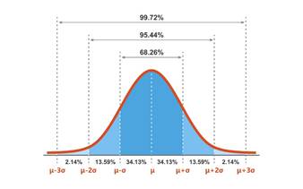
The Normal Distribution: Setting Merit Scholarships

Defined by a Mean (μ) and a Variance (σ²)

Life Case: The Presidential Scholarship

The VP of Finance tells you, ” We can only afford to give the top Presidential Scholarship to the top 20% of the applicant pool.” You need to determine the GPA cutoff for this award.

• The average GPA of your applicant pool (μ) is 3.40.
• Using Excel’s Formula STDEV.P(“Name of the column with all GPAs of admitted students”), you calculated that the Standard Deviation (σ) of the entire admitted group is 0.40.
• Using either Excel formula NORM.S.INV(0.80) or a a Z-Table (look for the value closest to 0.8000) you will find out that the Z-score for the top 20% is approximately 0.84. (This means the cutoff is 0.84 standard deviations above the average).

The Calculation:

Cutoff= mean+(Zscore*Standard Deviation) = 3.4 + 0.84 *0.4 = 3.74

Strategy: you set the scholarship GPA requirement at 3.74. By using the properties of the Normal Distribution, you can confidently predict that roughly 20% of your applicants will qualify, allowing you to project your financial aid discount rate accurately before a single award letter is mailed.

Probability theory offers a “menu” of distribution patterns that describe how random variables behave. Four of these are particularly relevant to the student funnel.

Now lets solve the following problems:

Scenario 1: We spent $20,000 on a digital campaign targeting “STEM Interest” students. Historically, the application rate for our general inquiry pool is 10%. We had 5,000 students in the STEM campaign. 600 of them applied.  We want to know if the campaign actually influenced behavior or if these students would have applied anyway. Using conditional probability, determine if the campaign worked.

Scenario 2: The President wants a precise forecast for the incoming class size. We cannot use a single yield rate because Locals (1,000 admits, historic yield is 30%) and Out-of-State students (2,000 admits and historic yield is 10%) behave differently. Using the Law of Total Probability, what is the total expected size of the incoming class?

Scenario 3: We have admitted 2,500 students. Our historical yield rate is 20%. We have exactly 525 beds in the residence halls. Do we risk overfilling the 525 beds?

Scenario 4: During the week before the deposit deadline, we expect a surge in phone calls. Historical data shows we average 16 calls per hour. We want to staff enough student workers to handle “Peak Volume.” How many calls per hour should we staff for?